Time-to-event
Survival analysis: Kaplan-Meier, Cox regression, assumptions and competing risks
Under development.
Time-to-event analysis (survival analysis) looks at the time until an event and handles the fact that not everyone reaches the event during follow-up (censoring). It is the typical framework for a cohort study with an outcome over time.
The code examples use generic path and variable names. Adapt them to your project. The packages (survival, survminer, tidycmprsk) must be installed in your R environment on DST.
Starting point
You need two things per person: follow-up time (how long the person was followed) and event status (whether the event/outcome occurred in that time: 1 = yes, 0 = censored, i.e. not seen during follow-up). Follow-up time is stop date minus index date, where the stop date is the first of outcome, death, emigration or end of study; see Calculate follow-up time and event variable in Phase 12 for the construction itself.
library(survival) # Surv(), survfit(), coxph(), cox.zph()

df <- readRDS("path/to/analysis.rds") # analysis-ready dataset, one row per person

# Surv() combines time + status into one "survival object" used by all the models:
#   time_days = days from index to event OR censoring (whichever comes first)
#   outcome   = 1 if the event occurred, 0 if the person was censored
# We build the object here ONLY to see what Surv() produces:
survival_obj <- Surv(time = df$time_days, event = df$outcome)
survival_obj # view the object: a "+" marks a censored person (e.g. 12+)

# In practice you don't need to store it: in the models below you write
# Surv(...) directly in the formula. It is shown here only for understanding.
Kaplan-Meier curves
survfit() computes the Kaplan-Meier estimate (the event-free proportion over time), and ggsurvplot() draws it nicely.
library(survminer) # ggsurvplot()

fit <- survfit(
  Surv(time_days, outcome) ~ exposure, # one curve per exposure group
  data = df
)

ggsurvplot(
  fit,
  data = df,
  pval = TRUE, # show the log-rank test p-value
  conf.int = TRUE, # show confidence bands around the curves
  risk.table = TRUE, # table below the figure: number at risk over time
  xlab = "Days since index", # axis labels
  ylab = "Event-free proportion"
)
With simulated numbers the curves look like this (here the exposed drop faster, i.e. they get the outcome more often):
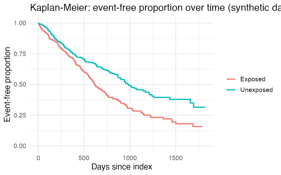
ggsurvplot() typically also adds a risk table below the figure.Kaplan-Meier can overestimate the risk if a competing event (typically death) can preclude your outcome - see Competing risks below.
Cox regression (hazard ratio)
coxph() gives hazard ratios (HR) adjusted for covariates. tbl_regression(exponentiate = TRUE) shows them as HRs instead of log-hazards.
library(gtsummary) # tbl_regression()

# Without replacement (each person appears only once): an ordinary Cox model.
cox <- coxph(Surv(time_days, outcome) ~ exposure + age + sex, data = df)

cox %>% # pass the model on to a clean table
  tbl_regression(exponentiate = TRUE) # exponentiate = TRUE -> hazard ratios
A hazard ratio reads like an OR/RR: 1 = no difference, above 1 = higher rate, below 1 = lower. See Reading your result.
The difference with replacement. If the comparison cohort is matched with replacement (or there is crossover), the same person appears several times and the rows are not independent. Then you add one single argument - cluster = pnr - to exactly the same model. It does not change the hazard ratio estimate (the HR is the same); it only corrects the standard errors and confidence intervals, which would otherwise be artificially narrow. Same idea as in Regression.
# With replacement (same person several times): the ONLY difference from the model above is cluster = pnr.
coxph(
  Surv(time_days, outcome) ~ exposure + age + sex,
  data = df,
  cluster = pnr
) %>% # <- the only change: cluster on person id
  tbl_regression(exponentiate = TRUE) # HR unchanged; only the CIs become correct (usually wider)
Note the syntax: coxph() takes the cluster variable as an argument without a tilde (cluster = pnr), whereas sandwich::vcovCL() on the Regression page uses a formula with a tilde (cluster = ~ pnr). Same idea (cluster on person id), just two functions’ different ways of receiving the variable.
What is your time scale? The time axis (what the x-axis shows on e.g. a Kaplan-Meier curve) is a choice. By default it is time since index - how long each person has been followed since their own start date (that is time_days in the examples). But you can also follow people on:
- attained age - so the model compares people at the same age. That adjusts for age automatically and flexibly (a strong confounder for most outcomes), without you having to model the shape of age yourself. Common in register studies.
- calendar time - if the calendar period itself matters (e.g. treatment that has changed over the years).
Time since index is simplest; age-as-time-scale is often stronger when risk is driven heavily by age. Technically you choose the time scale via what you put in as time in Surv().
Check the assumption: proportional hazards
The Cox model assumes proportional hazards (PH): that a variable’s effect is constant over time. If it does not hold, the single hazard ratio is misleading. Always check it with cox.zph(), which is based on Schoenfeld residuals (in short, a measure of whether the effect “drifts” over time).
ph <- cox.zph(cox) # formal PH test per variable + global
print(ph) # small p-value = sign the assumption is VIOLATED
plot(ph) # residual curve per variable; a sloping curve
#   indicates a non-proportional hazard
What to do if the assumption is violated
If a variable violates the assumption, you can e.g. stratify on it (+ strata(variable) in the model, giving it its own baseline hazard) or model a time-dependent effect (let the effect change over follow-up).
A third alternative is to drop the hazard ratio and use RMST (restricted mean survival time): the average event-free time within a fixed window (e.g. “months alive within 5 years”). You compare groups by the difference in RMST, measured in time units instead of a ratio, and it is valid even when PH is violated. In R: the survRM2 package.
Competing risks
If another event can preclude your outcome (classically: death, before the outcome can occur), it is a competing risk. A plain Kaplan-Meier then overestimates the risk, because it treats those who died as merely censored. This is the rule rather than the exception in register cohorts with older people or long follow-up.
The idea is simple: each person ends up in one of three places, and only the first thing that happens counts - (1) they never reach an event during follow-up (censored), (2) they get your outcome, or (3) they are hit by the competing event (e.g. death). Someone who dies first can never reach the outcome, and the analysis must reflect that.
1. Set up the data
You need the same two variables as for an ordinary Cox model - but the status variable now takes three values instead of two (so we call it status instead of outcome):
time_days- the time from index to the first thing that happens (outcome, death or end of follow-up).status- what happened: censored, outcome or death.
status must be a factor, and tidycmprsk requires “censored” to be the first level. The order of the levels is also where you tell R which level is your outcome and which is the competing risk:
library(tidycmprsk) # cuminc(), crr()

df <- df %>%
  mutate(
    status = factor(
      status_code, # your raw code, one value per person (e.g. 0/1/2)
      levels = c(0, 1, 2), # the order sets the meaning:
      labels = c(
        "censored", #   1st level = censored (MUST be first)
        "outcome", #   2nd level = your outcome (the one crr models)
        "death"
      ) #   3rd level = the competing risk
    )
  )
You build status_code (0/1/2) from the dates - what happened first: 0 = censored (e.g. end of follow-up, emigrated or otherwise lost), 1 = outcome, 2 = death. The construction lives in Calculate follow-up time and event variable (Phase 12). The number you give censoring does not matter - what matters is that the censored level is listed first in levels = (which is why it is 0 here).
2. Describe the risk over time (CIF)
Instead of Kaplan-Meier, use the cumulative incidence function (CIF, also called Aalen-Johansen). It allocates people correctly across the competing outcomes, so death no longer “steals” risk from the outcome. (This is about the curve; the regression itself is still done with Cox, see step 3.)
# Surv(time, status) with the factor status -> cumulative incidence for EACH event type:
cuminc(
  Surv(time_days, status) ~ exposure, # one curve per exposure group
  data = df
) # also gives Gray's test for a group difference
3. Regression: pick the model to match your question
Cox can absolutely be used - you just need to know which of two questions you are asking:
- Etiology (the rate of the outcome): run an ordinary Cox, but censor the competing event. You do that by setting the event to
status == "outcome": both censored and dead people then become “no event”. This is the cause-specific hazard. - Absolute/cumulative risk: use Fine-Gray (
crr), where the dead stay in the risk set.crrby default models the first event type after “censored” (here “outcome”) and treats the rest (“death”) as competing. This is the subdistribution hazard.
# Etiology - cause-specific Cox: status == "outcome" turns death (and censored) into "no event"
coxph(
  Surv(time_days, status == "outcome") ~ exposure + age + sex,
  data = df
) %>%
  tbl_regression(exponentiate = TRUE) # -> cause-specific hazard ratio

# Absolute risk - Fine-Gray: uses the factor status directly (outcome vs. competing)
crr(Surv(time_days, status) ~ exposure + age + sex, data = df) %>%
  tbl_regression(exponentiate = TRUE) # -> subdistribution hazard ratio
Rule of thumb: which one do I pick?
If you want to describe or predict risk (e.g. “what is the 5-year risk of the outcome?”), use CIF + Fine-Gray. If you want to understand a causal relationship (e.g. “does the exposure raise the rate of the outcome?”), use the cause-specific Cox. Many studies report both.
Time-varying covariates (briefly)
If a variable changes during follow-up (e.g. a blood test or BMI), it cannot be a single value per person. It must be in start/stop format (one row per interval), built with survival::tmerge() and analysed with coxph(Surv(tstart, tstop, outcome) ~ ...). The reshaping itself is in Time-varying variables.
Remember: anything leaving DST must go through output control - no small cells, only aggregated results. See Phase 14 - Export and repatriation.
Further depth in The Epidemiologist R Handbook: