Choosing a statistical analysis
Overview: which test or model fits your data?
Under development - needs further review. Use the page as a quick pointer, not the final word: always check the assumptions and your analysis plan, and look things up if in doubt. An interactive “click your way through” version is on the way.
Start with your question. First state your research question and null hypothesis - they drive everything else.
In the R commands in the tables, x, y, group, m0 etc. are placeholders - replace them with your own variable and value names. Commands written as package::function (e.g. survival::coxph, epitools::riskratio) come from a package that must be installed on DST; the rest are base R (the stats package, always available). Regression and time-to-event are expanded in Regression and Time-to-event.
Prefer a flowchart? Antoine Soetewey’s decision tree for choosing a statistical test is an excellent visual companion to the tables here - you click through data type, number of groups, paired/unpaired and distribution.
Find the right test - three questions:
- What data type is your outcome? Numeric (a number), binary (yes/no) or time-to-event (time until an event). This picks the tab below.
- Are your data paired or unpaired? The same person measured several times or in 1:1 matched pairs = paired; otherwise unpaired. This picks the row in the table.
- Are the assumptions for a parametric test met? If they are, use the parametric one; otherwise the nonparametric counterpart. This picks between the two rows in each block.
New to the concepts? Expand them under Concepts in brief at the bottom.
| Analysis type | Paired? | Purpose | Parametric? | Test | Assumptions | R |
|---|---|---|---|---|---|---|
| Mean, one group | Irrelevant | Compare one group to a hypothetical value | Parametric | One-sample t-test | Normal distribution; independent |
t.test(x, mu = m0)
|
| Nonparametric | Wilcoxon signed-rank | Symmetric distribution about the median; independent |
wilcox.test(x, mu = m0)
|
|||
| Mean, two groups | Unpaired | Compare two unpaired groups | Parametric | Unpaired t-test | Normal in both; (equal variance); independent |
t.test(y ~ group)
|
| Nonparametric | Mann-Whitney (rank-sum) | Independent; same distribution shape |
wilcox.test(y ~ group)
|
|||
| Paired | Compare two paired groups | Parametric | Paired t-test | Normally distributed paired differences |
t.test(x1, x2, paired = TRUE)
|
|
| Nonparametric | Wilcoxon signed-rank | Symmetric paired differences; independent |
wilcox.test(x1, x2, paired = TRUE)
|
|||
| Regression | Unpaired | General linear model for the mean | Parametric | Linear regression | Normal distribution; independent |
lm(y ~ x)
|
| Mean, several groups | Unpaired | Compare several means | Parametric | One-way ANOVA | Normal distribution; independent |
aov(y ~ group)
|
| Nonparametric | Kruskal-Wallis | Independent; same distribution shape |
kruskal.test(y ~ group)
|
|||
| Relationship (correlation) | Irrelevant | Describe the relationship between two continuous variables | Parametric | Pearson correlation | Linear relationship; normal; independent |
cor.test(x, y)
|
| Nonparametric | Spearman rank correlation | Monotonic relationship; independent |
cor.test(x, y, method = “spearman”)
|
| Analysis type | Paired? | Purpose | Parametric? | Test | Assumptions | R |
|---|---|---|---|---|---|---|
| Proportion, one group | Irrelevant | Compare one group to a hypothetical value | Parametric* | Binomial test | Binomial distribution; independent |
binom.test(x, n, p = p0) (exact); prop.test(x, n, p = p0) (approx.)
|
| Proportion, two groups | Unpaired | Compare two unpaired groups | Parametric* | Chi-square / Fisher’s exact | Independent (Fisher for small counts) |
chisq.test(table); fisher.test(table)
|
| Paired | Compare two paired groups | Parametric* | McNemar | Paired obs.; independent pairs |
mcnemar.test(table)
|
|
| Regression | Unpaired | Binary regression for relative risk | Parametric | Log-binomial regression | Binomial; probability modelled by covariates |
glm(y ~ x, family = binomial(link = “log”))
|
* Chi-square, Fisher’s exact, McNemar and the binomial test are called nonparametric in many textbooks (they assume no normal distribution). Here Parner’s scheme is followed, where “parametric” means the test assumes a specific distribution - for these tests the binomial.
An effect measure with a confidence interval for two groups (risk difference, RR, OR) is a descriptive measure, not a hypothesis test - compute it with e.g. epitools::riskratio() or epitools::oddsratio().
Log-binomial regression in the table = a glm with a log link, estimating relative risk (RR) instead of an odds ratio.
| Analysis type | Paired? | Purpose | Parametric? | Test | Assumptions | R |
|---|---|---|---|---|---|---|
| Cumulative risk | Irrelevant | Estimate the cumulative risk / compare groups | Nonparametric | Kaplan-Meier + log-rank | Independent; independent right censoring |
survival::survfit(Surv(time, event) ~ group); survival::survdiff(Surv(time, event) ~ group)
|
| Rate / hazard ratio | Unpaired | Compare rates | Semi-parametric | Cox regression | Independent; independent right censoring; proportional hazards |
survival::coxph(Surv(time, event) ~ x); PH check: survival::cox.zph()
|
Working with rates per person-year? If you compare incidence rates split by e.g. age groups or calendar periods (rather than time-to-first-event), you use Poisson regression, which gives an incidence rate ratio (IRR). See Rates and rate ratios (Poisson) for when to choose it over Cox.
Concepts in brief (click to expand)
New to statistics? Expand for the concepts the tables build on.
Which data type is my outcome?
The data type decides which table you need:
- Numeric (continuous): a number, e.g. age, BMI or blood pressure.
- Binary (dichotomous): yes/no, e.g. whether a person got a diagnosis or not.
- Time-to-event: the time until an event happens, where not everyone reaches it during follow-up (censoring) - e.g. time to diagnosis or death.
What is a normal distribution?
A normal distribution is bell-shaped: most values lie in the middle, with few very small or very large ones. A skewed (or irregular) distribution does not - it may have a long tail to one side.
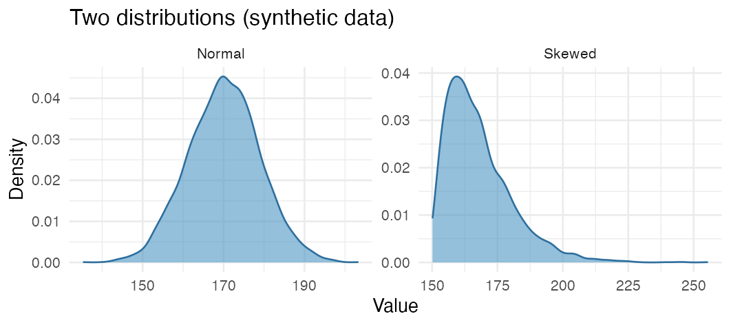
Most parametric tests (e.g. t-test) assume the data are roughly normal; if they are clearly skewed, that points to a nonparametric test. Check the shape with a histogram (hist()) or a Q-Q plot (qqnorm() + qqline()).
Mean or median?
The mean can be pulled by extreme values (outliers), while the median (the middle value) is more robust. In a right-skewed distribution the mean therefore sits to the right of the median:
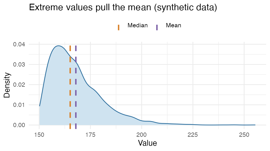
Parametric tests typically work with the mean; nonparametric tests use ranks/median and are therefore less sensitive to outliers and skew.
Dependent vs. independent variable
- A dependent variable is your outcome - the result you are studying (e.g. weight loss).
- An independent variable is something you have measured that might affect the outcome (e.g. treatment, sex, age). In a study of two diets, weight loss is the dependent variable and diet an independent variable.
(Don’t confuse “independent variable” with “independent data” - see the next box.)
Paired or unpaired data
- Unpaired or independent data: different, unrelated people in each group (e.g. one group gets diet 1, another diet 2). Recording e.g. sex on each person does not make it paired - sex and outcome are just two different variables.
- Paired/dependent data: the same unit is measured more than once (e.g. weight before and after a treatment) or forms 1:1 matched pairs. This decides whether you use a paired or unpaired test (see the tables).
Paired and matched are not the same
A 1:1 matched pair (one case + one matched control) corresponds to paired data and is analysed as paired. But if you match with several controls (e.g. 1:5 case-control) or have a matched cohort, there are matched sets with more than two members each - a paired test needs pairs and so does not fit. They are analysed instead with conditional logistic regression (clogit + strata(), see Regression) or stratified/clustered Cox (see Time-to-event), which generalise the pairing idea to matched sets of any size.
Parametric or nonparametric
A parametric test or model assumes a particular distribution - usually the normal for tests on numbers, or the binomial for tests on proportions. A nonparametric test assumes no particular distribution and instead works on the ranks of the values (e.g. Wilcoxon); it is more robust to skewed distributions and outliers, but usually has slightly less power. Rule of thumb: if the parametric test’s assumptions hold (see Assumptions below), use it; otherwise the nonparametric one. (Cox is called semi-parametric: it assumes no particular distribution for the survival time, but a fixed structure for how covariates affect the risk.)
The nonparametric “twin” of each t-test
Each t-test has a nonparametric counterpart, used when the normality assumption does not hold:
- One-sample t-test → one-sample Wilcoxon signed-rank (tests the median against a value)
- Unpaired t-test → Mann-Whitney U (= Wilcoxon rank-sum; two independent groups)
- Paired t-test → Wilcoxon signed-rank (paired measurements)
Mind the names: Mann-Whitney U is also called Wilcoxon rank-sum - not the same as Wilcoxon signed-rank (the paired/one-sample one). In R both are wilcox.test(); the difference is paired = and whether you give two groups or two measurements.
Assumptions
Assumptions behind the tests - click for details
Every test rests on some assumptions. Some you can test or inspect in the data; others are design questions you must judge from how the data were collected. Here are the ones named in the tables:
Normal distribution (t-tests, linear regression, ANOVA). That the values - or for regression the model’s residuals - are roughly normally distributed. Check: visually with a histogram (hist()) and Q-Q plot (qqnorm() + qqline()); optionally a formal test (shapiro.test()), but it is oversensitive in large samples, so trust the visual most. With large samples, t-tests and means are also robust (the central limit theorem).
Normally distributed paired differences (paired t-test). It is the differences (e.g. before minus after) that should be roughly normal - not each group separately. Check: histogram/Q-Q plot of the differences.
Symmetric distribution (Wilcoxon signed-rank). The test assumes the distribution of the values (about the median) or of the paired differences is symmetric - not necessarily normal. Check: histogram of the values/differences; if it is clearly skewed, a sign test may be more appropriate.
Equal variance (homoscedasticity) (unpaired t-test, ANOVA, linear regression). The groups (or residuals) have roughly the same spread. Check: boxplot per group; var.test() (two groups) or car::leveneTest() (several groups); for regression a residual plot via plot(model). Note: Welch’s t-test (R’s default) does not assume equal variance, so it is rarely a problem there.
Independent observations (almost all tests). Each observation contributes independent information - e.g. not several rows from the same person or other clusters. Cannot be tested in the data - it is a design / data-structure question. Inspect: do you have repeated rows per person, matched pairs or clusters? Then use a method that accounts for it (paired test, clustered standard errors - see Regression - or a mixed model).
Same distribution shape (nonparametric tests: Wilcoxon, Mann-Whitney, Kruskal-Wallis). For the comparison to be meaningful, the groups should have roughly the same distribution shape. Check: compare density curves/histograms or boxplots per group (hard to test formally, so inspect visually).
Binomial distribution (binomial test). A yes/no outcome counted over independent units with the same probability. Mostly a design question - judge whether the data fit it (independent people, same outcome definition).
Adequate expected cell counts (chi-square). The test is unreliable if the expected counts in the cells are too small (rule of thumb: below 5). Check: look at the expected counts with chisq.test(table)$expected; if some are small, use fisher.test() instead.
Independent pairs (McNemar). The pairs are matched, and the pairs themselves are independent of each other. Design question - follows from how you paired.
Independent (right) censoring (Kaplan-Meier, log-rank, Cox). That those who are censored (e.g. lost to follow-up) do not systematically have higher or lower risk than those still followed. Cannot be tested directly - argue from why people are censored (administrative end of follow-up = typically independent; loss to follow-up tied to health = problematic). Sensitivity analyses if needed.
Proportional hazards (Cox regression). That a variable’s effect (hazard ratio) is roughly constant over time. Check: survival::cox.zph() (Schoenfeld residuals) and log-log survival curves - see Time-to-event.
Remember: anything leaving DST must go through output control - no small cells, only aggregated results. See Phase 14 - Export and repatriation.
This overview is based on notes from Erik Parner’s statistics courses at Aarhus University - courses I warmly recommend.
Further depth in The Epidemiologist R Handbook:
New to the underlying statistics (what a test, p-value or confidence interval actually means)? See Learning Statistics with R (Navarro) - a beginner-friendly walkthrough of the theory behind them.